Física e controle de um simulador PID de HVAC

Uma explicação intuitiva de engenharia sobre a física térmica, o comportamento da água gelada, o controle PID e a medição de energia em um simulador interativo de unidades fan coil e unidades de tratamento de ar.

Published: Aug 26, 2026
By: Ricardo Rosal"
Reading: 26 minutes

Malha de controle de HVAC com temperatura do ar, válvula de água gelada, controlador PID e gráficos de tendência em tempo real

Abstract

Este artigo explica o modelo de engenharia por trás de um simulador interativo de controle de HVAC para unidades fan coil e unidades de tratamento de ar. Apresenta as equações de transferência de calor do lado do ar e da água gelada, explica como a posição da válvula afeta a capacidade de resfriamento, descreve o controlador PID discreto usado para regular a temperatura do ar de insuflação e relaciona a carga térmica resultante à demanda elétrica, ao consumo de energia e ao custo operacional.

Um controlador só é útil quando seu comportamento é compreendido em conjunto com o processo que ele tenta controlar.

— Princípio da engenharia de controle

Acesso ao simulador#

Simulador HVAC Lab

O que o simulador representa#

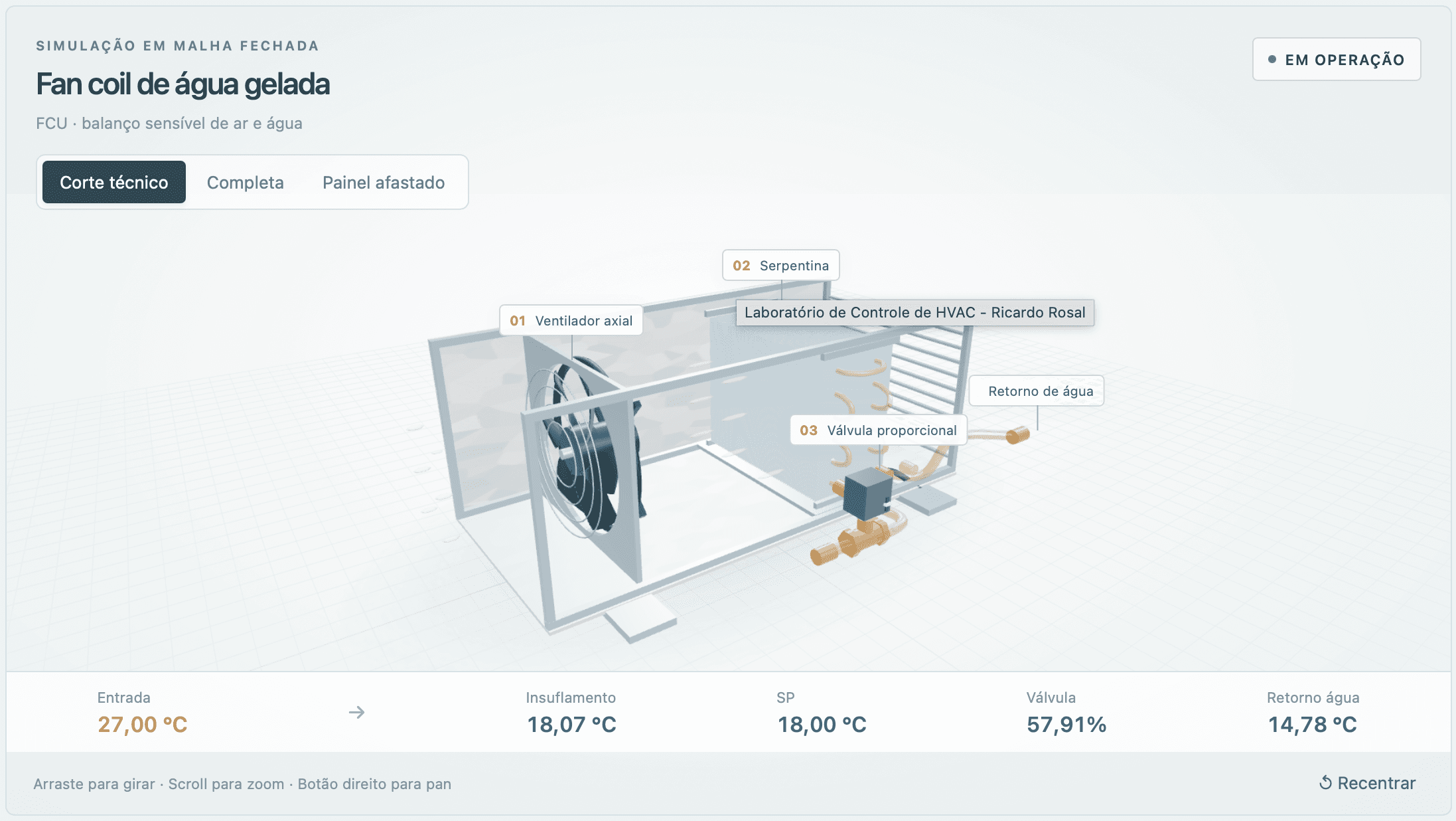
O simulador modela um sistema simplificado de HVAC — aquecimento, ventilação e ar-condicionado — com água gelada, no qual o ar passa por uma serpentina de resfriamento antes de ser insuflado em um ambiente climatizado.

As duas configurações predefinidas de equipamento representam o mesmo processo físico em escalas diferentes.

Uma unidade fan coil, ou FCU (Fan Coil Unit), normalmente atende a uma zona menor e, por isso, opera com vazões de ar e de água gelada relativamente baixas. Uma unidade de tratamento de ar, ou AHU (Air Handling Unit), representa um sistema maior, com vazões de ar e de água e capacidade de resfriamento substancialmente superiores.

A malha básica de controle é

\text{Setpoint de temperatura} \rightarrow \text{Controlador PID} \rightarrow \text{Válvula de água gelada} \rightarrow \text{Serpentina de resfriamento} \rightarrow \text{Temperatura do ar de insuflação}.

A temperatura do ar de insuflação é medida continuamente e realimentada ao controlador.

Se o ar estiver mais quente que o valor de referência (setpoint), o controlador abre a válvula de água gelada. Mais água gelada circula pela serpentina, que absorve mais calor, e a temperatura do ar de insuflação diminui.

Se o ar ficar mais frio que o necessário, o controlador reduz a abertura da válvula.

O balanço de energia do lado do ar#

O resfriamento começa com o calor sensível transportado pelo ar.

Para uma corrente de ar que passa pela serpentina de resfriamento, a taxa de resfriamento sensível pode ser aproximada por

\dot{Q}_{air} = \dot{m}_{air} c_{p,air} \left( T_{inlet}-T_{supply} \right).

Nessa expressão,

$\dot{Q}_{air}$ é a taxa de resfriamento sensível em kW,
$\dot{m}_{air}$ é a vazão mássica de ar em kg/s,
$c_{p,air}$ é o calor específico do ar,
$T_{inlet}$ é a temperatura de entrada do ar na serpentina,
$T_{supply}$ é a temperatura de saída do ar da serpentina.

O simulador converte a vazão volumétrica de ar em vazão mássica usando

\dot{m}_{air} = \rho_{air}\dot{V}_{air},

em que a massa específica do ar é aproximada por

\rho_{air}\approx1.2\ \text{kg/m}^3.

O calor específico do ar é aproximado por

c_{p,air}\approx1.005\ \text{kJ/(kg·K)}.

Suponha que uma AHU movimente

\dot{V}_{air}=2.5\ \text{m}^3/\text{s}

e resfrie o ar de

26^\circ C

para

16^\circ C.

A vazão mássica é aproximadamente

\dot{m}_{air} = 1.2(2.5) = 3.0\ \text{kg/s}.

A taxa de resfriamento passa a ser

\dot{Q}_{air} = 3.0 \times 1.005 \times (26-16),

ou aproximadamente

30.2\ \text{kW}.

Isso ilustra por que a vazão de ar tem um efeito tão forte sobre a capacidade da serpentina. Resfriar o ar pela mesma diferença de temperatura com o dobro da vazão exige aproximadamente o dobro da taxa de resfriamento sensível.

O lado da água gelada#

A serpentina de resfriamento recebe água gelada de uma central de água gelada ou de um chiller.

O simulador representa o balanço térmico do lado da água por meio de

\dot{Q}_{CHW} = \dot{V}_{CHW} \rho_{water} c_{p,water} \left( T_{CHWR}-T_{CHWS} \right).

Os termos são

$\dot{V}_{CHW}$ : vazão volumétrica de água gelada,
$\rho_{water}$ : massa específica da água,
$c_{p,water}$ : calor específico da água,
$T_{CHWS}$ : temperatura de alimentação da água gelada,
$T_{CHWR}$ : temperatura de retorno da água gelada.

Aproximações típicas são

\rho_{water} \approx 1000\ \text{kg/m}^3

e

c_{p,water} \approx 4.186\ \text{kJ/(kg·K)}.

Assim, a água pode transportar uma grande quantidade de energia térmica com uma vazão relativamente modesta.

Por exemplo, uma vazão de água de

1\ \text{L/s}

com um aumento de temperatura de

5^\circ C

transporta aproximadamente

\dot{Q} = 0.001 \times 1000 \times 4.186 \times 5,

o que resulta em

\dot{Q} \approx 20.9\ \text{kW}.

Essa relação é uma das razões pelas quais os sistemas de água gelada são tão eficazes na distribuição de resfriamento em grandes edifícios.

A válvula de controle#

A válvula de água gelada é o atuador comandado pela malha PID.

Na forma mais simples, o simulador pode representar a vazão de água como

\dot{V}_{CHW} = \frac{u_{valve}}{100} \dot{V}_{max},

em que

u_{valve} \in [0,100].

Um comando de válvula de 50% produz, portanto, aproximadamente 50% da vazão máxima quando a característica selecionada para a válvula é linear.

As válvulas de controle reais costumam apresentar um comportamento mais complexo.

Uma válvula de igual porcentagem proporciona variações relativamente pequenas de vazão em baixas aberturas e variações cada vez maiores à medida que se aproxima da abertura total.

Uma relação simplificada de igual porcentagem pode ser escrita como

f(u) = \frac{R^{u}-1}{R-1},

em que $u$ é normalizado entre 0 e 1 e $R$ representa a rangeabilidade da válvula.

Essa diferença tem consequências importantes para o controle.

Uma válvula linear pode produzir um controle relativamente agressivo em baixa carga, enquanto uma válvula de igual porcentagem pode proporcionar uma modulação mais fina em pequenas aberturas e maior capacidade à medida que se abre.

Por que a temperatura de insuflação não muda instantaneamente#

Se o controlador movimentasse a válvula e a temperatura do ar de insuflação mudasse imediatamente, a simulação teria um comportamento irrealista.

Sistemas reais de HVAC possuem inércia térmica.

O metal da serpentina, o volume de água, o volume de ar, os sensores e as superfícies do trocador de calor precisam de tempo para responder.

Por isso, o simulador utiliza uma resposta dinâmica, em vez de saltar diretamente para a temperatura teórica de regime permanente.

Uma representação comum de primeira ordem é

\tau \frac{dT}{dt} + T = T_{target},

em que $\tau$ é a constante de tempo térmica.

Na forma discreta, a temperatura de insuflação pode ser atualizada aproximadamente por

T_{k+1} = T_k + \alpha \left( T_{target}-T_k \right),

com

\alpha = 1-e^{-\Delta t/\tau}.

Uma constante de tempo elevada produz uma resposta lenta da serpentina.

Uma constante de tempo pequena produz uma resposta mais rápida.

Esse modelo dinâmico aparentemente simples é fundamental, pois a sintonia PID só faz sentido quando o processo controlado possui uma dinâmica própria.

Efetividade da serpentina#

Normalmente, a serpentina de resfriamento não consegue reduzir a temperatura do ar de saída até a temperatura de alimentação da água gelada.

Em vez disso, o simulador calcula uma temperatura-alvo efetiva para o ar de saída com base na capacidade de resfriamento disponível e na efetividade da serpentina.

Um modelo conceitual simplificado é

T_{target} = T_{inlet} - \varepsilon \left( T_{inlet}-T_{CHWS} \right),

em que

0\leq\varepsilon\leq1

representa a efetividade da serpentina.

Se

\varepsilon=0,

a serpentina não fornece resfriamento.

Se

\varepsilon=1,

a temperatura teórica do ar de saída se aproxima da temperatura da água gelada na entrada.

Na prática, a efetividade depende de diversas variáveis que interagem entre si, incluindo as vazões de ar e de água, a geometria da serpentina, os coeficientes de transferência de calor e a diferença de temperatura entre os dois fluidos.

O simulador combina esses efeitos em um modelo dinâmico simplificado, adequado ao estudo do comportamento do controle sem exigir uma simulação completa do trocador de calor por volumes finitos.

O erro na malha de realimentação#

O objetivo do controlador é manter a temperatura do ar de insuflação próxima de um setpoint escolhido pelo usuário.

O erro de controle é definido como

e(t) = T_{supply}(t) - T_{setpoint}.

Essa convenção de sinais é adequada ao controle de resfriamento com ação direta.

Por exemplo, se

T_{supply}=20^\circ C

e

T_{setpoint}=16^\circ C,

então

e=4^\circ C.

O ar está quente demais, portanto o controlador deve aumentar o resfriamento.

Se

T_{supply}=15^\circ C,

então

e=-1^\circ C.

O ar está mais frio que o necessário, portanto o controlador deve fechar a válvula.

O controlador PID#

O simulador implementa um controlador PID discreto.

A forma conceitual contínua é

u(t) = K_p e(t) + K_i \int e(t)\,dt + K_d \frac{de(t)}{dt}.

Os três termos desempenham funções diferentes.

Ação proporcional#

A contribuição proporcional é

P=K_p e.

Um erro maior produz um comando de abertura maior para a válvula.

Se $K_p$ for muito pequeno, o sistema reage lentamente.

Se $K_p$ for muito elevado, o sistema pode se tornar agressivo e oscilatório.

Ação integral#

A contribuição integral acumula o erro passado:

I = K_i \int e(t)\,dt.

Sua principal finalidade é eliminar o desvio em regime permanente.

Suponha que apenas o controle proporcional estabilize a temperatura de insuflação em

16.8^\circ C

para um setpoint de

16^\circ C

Nesse caso,

permanece um pequeno erro.

O termo integral continua acumulando esse erro e aumenta gradualmente o resfriamento até que o desvio desapareça.

Ação derivativa#

O termo derivativo responde à taxa de variação do erro:

D = K_d \frac{de}{dt}.

Ele pode ser interpretado como um comportamento antecipatório.

Se a temperatura estiver se aproximando muito rapidamente do setpoint, a ação derivativa pode reduzir a saída do controlador antes que o sistema ultrapasse o valor desejado.

Em sistemas reais de HVAC, a ação derivativa costuma ser utilizada com cautela, pois o ruído de medição pode torná-la instável ou desnecessariamente sensível.

O cálculo do PID discreto#

Os computadores não resolvem a equação PID continuamente.

A simulação opera em intervalos discretos de tempo.

A cada passo de cálculo $\Delta t$ , o acumulador integral é atualizado aproximadamente por

I_k = I_{k-1} + e_k\Delta t.

A derivada pode ser aproximada por

\frac{de}{dt} \approx \frac{e_k-e_{k-1}}{\Delta t}.

A saída do controlador passa a ser

u_k = K_p e_k + K_i I_k + K_d \frac{e_k-e_{k-1}}{\Delta t}.

O comando resultante é limitado à faixa física da válvula:

0\% \leq u_k \leq 100\%.

O simulador utiliza um passo de cálculo da física da ordem de frações de segundo, permitindo que o comportamento transitório do controle permaneça suave, com baixo custo computacional no navegador.

Acúmulo excessivo da integral: windup#

Um controlador PID prático precisa lidar com a saturação do atuador.

Imagine que o ar de insuflação esteja extremamente quente e que o controlador calcule

u=180\%.

A válvula física não pode abrir além de 100%.

Se o termo integral continuar aumentando enquanto a válvula estiver saturada, ele pode atingir um valor muito elevado.

Mais tarde, mesmo depois que a temperatura atingir o setpoint, o controlador pode permanecer com a saída em 100%, porque a integral acumulada leva tempo para diminuir.

Esse fenômeno é chamado de windup integral.

O simulador evita o windup excessivo limitando ou atualizando condicionalmente o acumulador integral enquanto a saída do controlador está saturada.

Essa técnica é conhecida como anti-windup.

Sem anti-windup, os experimentos de resposta ao degrau podem produzir ultrapassagens do valor desejado irrealisticamente grandes e longos tempos de recuperação.

O que acontece após uma perturbação#

O simulador inclui uma função de perturbação em degrau, pois mudanças desse tipo estão entre as formas mais úteis de estudar sistemas de controle.

Considere um aumento abrupto de

+5^\circ C

na temperatura do ar de entrada.

Imediatamente após a perturbação,

T_{inlet}\uparrow.

A serpentina não consegue compensar instantaneamente, portanto

T_{supply}\uparrow.

Assim, o erro aumenta:

e = T_{supply}-T_{setpoint} \uparrow.

O controlador PID responde aumentando o comando da válvula:

u_{valve}\uparrow.

A vazão de água aumenta:

\dot{V}_{CHW}\uparrow.

A serpentina absorve mais calor:

\dot{Q}_{coil}\uparrow.

Com o tempo, a temperatura do ar de insuflação volta a se aproximar do setpoint.

Os gráficos de tendência permitem observar toda essa sequência.

Como ler o gráfico de temperatura#

O primeiro gráfico compara

T_{supply}

com

T_{setpoint}.

Um sistema bem sintonizado normalmente se aproxima do setpoint de forma suave.

Entre os comportamentos importantes a observar estão:

Tempo de subida ou de resposta — a rapidez com que o sistema reage após uma perturbação.

Sobressinal (overshoot) — quanto a temperatura controlada ultrapassa o valor desejado.

Tempo de acomodação — quanto tempo o sistema leva para permanecer próximo do setpoint.

Erro em regime permanente — a existência de um desvio persistente depois que o transitório desaparece.

Essas são medidas usuais de desempenho de sistemas de controle.

Como ler o gráfico de controle#

O segundo gráfico de tendência mostra o erro do controlador e a posição da válvula.

Se o erro for grande e positivo, a válvula geralmente deve se mover no sentido de abertura.

À medida que a temperatura se aproxima do setpoint, a válvula deve se estabilizar na posição intermediária necessária para equilibrar a carga térmica.

Uma válvula que permanece continuamente em 100% pode indicar que o ponto de operação solicitado excede a capacidade da serpentina modelada.

Uma válvula que oscila repetidamente entre valores altos e baixos pode indicar uma sintonia PID excessivamente agressiva.

Uma resposta lenta da válvula, combinada com um erro persistente, pode indicar ação proporcional ou integral insuficiente.

Como ler o gráfico de vazão e potência#

O terceiro gráfico relaciona o comportamento do controle ao comportamento energético.

O movimento da válvula altera a vazão de água gelada.

A vazão de água gelada altera a capacidade de resfriamento.

A carga de resfriamento influencia a potência elétrica do chiller.

Isso cria uma cadeia importante de relações de engenharia:

\text{Saída do PID} \rightarrow \text{Vazão de água} \rightarrow \text{Carga térmica} \rightarrow \text{Potência do chiller}.

Portanto, o controlador faz mais do que controlar a temperatura.

Ele influencia indiretamente o consumo de energia da central.

COP do chiller#

O simulador converte a carga de resfriamento em uma demanda elétrica aproximada usando o coeficiente de desempenho do chiller, ou COP.

O COP é definido como

COP = \frac{\dot{Q}_{thermal}}{P_{electrical}}.

Portanto,

P_{electrical} = \frac{\dot{Q}_{thermal}}{COP}.

Suponha que a serpentina exija

35\ \text{kW}

de potência térmica de resfriamento e que o COP do chiller seja

5.

A potência elétrica correspondente é aproximadamente

P_{electrical} = \frac{35}{5} = 7\ \text{kW}.

Um COP maior significa que se produz mais resfriamento para cada unidade de energia elétrica.

Acúmulo de energia#

A potência elétrica descreve a taxa instantânea de uso de energia.

O consumo de energia é a integral da potência ao longo do tempo.

Para um intervalo de simulação $\Delta t$ medido em segundos,

\Delta E = P_{electrical} \frac{\Delta t}{3600}.

A energia acumulada é

E = \sum P_{electrical} \frac{\Delta t}{3600}.

O resultado é expresso em

\text{kWh}.

Isso permite relacionar diretamente o comportamento do controle no curto prazo ao consumo de energia no longo prazo.

Custo monetário de operação#

Uma vez conhecida a energia elétrica, o custo estimado é calculado a partir da tarifa de eletricidade.

Se a tarifa for

r \quad [\$/\text{kWh}],

então

Cost = E r.

Por exemplo, se a simulação acumular

12\ \text{kWh}

e a eletricidade custar

\$0.18/\text{kWh},

o custo estimado de energia será

12\times0.18 = \$2.16.

Essa relação simples ajuda a conectar a engenharia de controle aos aspectos econômicos da operação.

Um controlador que mantém a temperatura adequadamente, mas causa oscilações excessivas, pode aumentar a movimentação da válvula e a demanda de resfriamento.

Portanto, a qualidade do controle e o desempenho energético estão relacionados.

Medição do volume de água gelada#

O simulador também integra a vazão de água gelada.

O volume acumulado é

V_{total} = \sum \dot{V}_{CHW}\Delta t.

Esse valor é exibido em metros cúbicos e também pode ser convertido em galões.

Ao contrário da energia elétrica, o volume de água gelada não é necessariamente uma grandeza usada diretamente para cobrança em todos os edifícios.

Ainda assim, ele é útil para compreender a demanda hidrônica e comparar cenários de operação.

Conversão da capacidade de resfriamento em toneladas de refrigeração#

Na prática de HVAC, a capacidade de resfriamento costuma ser expressa em toneladas de refrigeração.

A conversão aproximada é

1\ TR \approx 3.517\ \text{kW}_{thermal}.

Portanto,

TR = \frac{\dot{Q}_{thermal}}{3.517}.

Para uma carga térmica de

35.17\ \text{kW},

a capacidade correspondente é aproximadamente

10\ TR.

O simulador exibe ambas as unidades para que os usuários possam transitar entre os cálculos de engenharia no SI e a terminologia usual do setor de HVAC.

Comportamento da FCU em comparação com a AHU#

Embora as equações que regem o sistema sejam as mesmas, as configurações predefinidas produzem respostas perceptivelmente diferentes.

Uma FCU normalmente utiliza vazões de ar e de água menores.

Sua carga térmica é, portanto, comparativamente pequena.

Uma AHU opera em uma escala maior.

Uma vazão de ar maior significa que cada grau de redução de temperatura exige uma capacidade de resfriamento consideravelmente maior:

\dot{Q}_{air} \propto \dot{V}_{air}.

Consequentemente, parâmetros que funcionam bem para a FCU não garantem um comportamento dinâmico idêntico para a AHU.

Isso ilustra um princípio importante da engenharia de controle:

A sintonia PID pertence ao processo, não apenas ao controlador.

Os mesmos ganhos numéricos podem produzir comportamentos diferentes quando o equipamento controlado muda.

Por que alterar a vazão de ar modifica a malha#

O aumento da vazão de ar afeta o simulador de várias maneiras.

Para as mesmas temperaturas de entrada e de insuflação,

\dot{Q}_{air} = \rho \dot{V}_{air} c_p \Delta T.

Portanto,

\dot{V}_{air}\uparrow \Rightarrow \dot{Q}_{air}\uparrow.

A serpentina precisa remover mais calor.

Consequentemente, o controlador pode exigir uma abertura maior da válvula.

Se a vazão máxima de água gelada for insuficiente, o controlador pode atingir

100\%

sem alcançar o setpoint desejado.

Esse é um exemplo de saturação do atuador causada por capacidade insuficiente da instalação, e não por uma sintonia PID inadequada.

Por que a temperatura de alimentação da água gelada importa#

O potencial de resfriamento de uma serpentina depende fortemente da diferença de temperatura entre o ar e a água gelada.

Se a temperatura de alimentação da água gelada diminuir,

T_{CHWS}\downarrow,

a diferença de temperatura que impulsiona a transferência de calor geralmente aumenta.

Assim, a serpentina pode produzir mais resfriamento em condições semelhantes de vazão.

Por outro lado, elevar a temperatura de alimentação da água gelada pode melhorar a eficiência da central em muitas instalações reais, mas também reduzir a capacidade disponível da serpentina.

Isso cria um compromisso, no nível do sistema, entre o desempenho da serpentina e a eficiência do chiller.

O simulador permite explorar diretamente o lado térmico dessa interação.

Por que a vazão máxima de água importa#

A vazão máxima de água define o limite superior da capacidade de resfriamento disponível no modelo da válvula.

Se a válvula atingir 100%, então

\dot{V}_{CHW} = \dot{V}_{max}.

Se a transferência de calor necessária ainda exceder o que a vazão de água disponível pode atender, a temperatura do ar de insuflação não conseguirá atingir o valor desejado.

Aumentar os ganhos do PID não resolverá essa condição.

A limitação é física, não matemática.

A arquitetura com Web Worker#

A implementação no navegador separa a simulação numérica da interface principal em React.

A arquitetura é aproximadamente

Interface React
      │
      │ parâmetros
      ▼
Web Worker
      │
      ├── modelo térmico
      ├── controlador PID
      ├── cálculos hidrônicos
      └── medição de energia
      │
      │ telemetria
      ▼
Painel React
      │
      ├── valores digitais
      └── gráficos de tendência em Canvas

Essa separação é importante porque as interfaces de navegador normalmente são executadas na thread principal do JavaScript.

Se cálculos numéricos intensivos e a renderização dos gráficos compartilharem essa thread, a interação pode ficar lenta.

O Web Worker executa a simulação de forma independente.

A interface recebe mensagens periódicas de telemetria e as exibe sem realizar os cálculos físicos.

Passo de tempo da física e passo de tempo da exibição#

O simulador distingue intencionalmente a frequência de simulação da frequência de exibição.

O mecanismo de simulação física pode calcular com um passo de aproximadamente

\Delta t=0.2\ \text{s},

enquanto a telemetria é enviada ao painel visível com menor frequência.

Isso significa que o processo matemático pode manter uma resolução temporal razoavelmente fina sem obrigar o React e os gráficos a serem redesenhados cinco vezes por segundo.

O conceito é semelhante ao de um sistema real de automação predial.

Um controlador pode executar sua lógica interna com frequência, mesmo que a estação de operação registre ou represente os dados em gráficos a uma taxa menor.

Por que os gráficos usam Canvas#

Versões anteriores da aplicação utilizavam renderização de gráficos baseada em SVG.

O SVG é excelente para muitas aplicações com painéis, mas a atualização contínua de curvas de engenharia pode causar atualizações repetidas do DOM e dos traçados.

A versão atual desenha as curvas de tendência no Canvas do HTML.

O Canvas trata o gráfico principalmente como uma superfície de desenho em bitmap, em vez de manter uma grande hierarquia de elementos gráficos no DOM.

Para um simulador em execução contínua, isso proporciona uma estratégia de renderização mais simples e com uso mais eficiente de memória.

O buffer do histórico também tem um limite deliberado.

Quando o número máximo de amostras é atingido, as mais antigas são removidas.

Assim, a quantidade de dados dos gráficos permanece aproximadamente constante, mesmo que o simulador funcione por várias horas.

Velocidade da simulação#

O simulador oferece os seguintes modos de velocidade:

1\times,\quad2\times,\quad5\times

Esses modos permitem acelerar o tempo simulado.

Uma velocidade de simulação maior não exige que a interface do navegador seja redesenhada com uma frequência cinco vezes maior.

Em vez disso, o worker avança o tempo simulado mais rapidamente, enquanto a taxa de telemetria visível permanece controlada.

Isso preserva a capacidade de resposta da interface e reduz o trabalho desnecessário de renderização.

Para que o simulador é útil#

A aplicação é particularmente útil para desenvolver a intuição sobre relações que, de outra forma, poderiam parecer abstratas.

Os usuários podem observar experimentalmente como

o ganho proporcional afeta a rapidez da resposta,
o ganho integral elimina o desvio residual,
ganhos excessivos geram oscilação,
a inércia térmica atrasa a resposta,
a vazão de ar altera a capacidade de resfriamento necessária,
a vazão de água afeta o desempenho da serpentina,
a temperatura da água gelada afeta o resfriamento disponível,
as perturbações se propagam por uma malha de realimentação,
a saturação da válvula revela limitações de capacidade,
o COP relaciona a demanda térmica à demanda elétrica,
e as decisões de controle influenciam o custo acumulado de energia.

Essas relações são difíceis de compreender apenas pelas equações.

O simulador permite variar um parâmetro de cada vez e observar os efeitos em tempo real.

Experimento sugerido: controle proporcional#

Comece com

K_i=0

e

K_d=0.

Utilize apenas o controle proporcional.

Comece com um valor baixo de $K_p$ e observe a resposta da temperatura.

Aumente $K_p$ gradualmente.

Você deverá perceber que o controlador passa a responder mais rapidamente.

Com ajustes suficientemente agressivos, a oscilação ou o sobressinal podem se tornar mais pronunciados.

Observe também se a temperatura final de insuflação se estabiliza exatamente no setpoint.

Um erro residual é comum no controle exclusivamente proporcional.

Experimento sugerido: adição da ação integral#

Em seguida, introduza um pequeno ganho integral.

Observe como o controlador corrige lentamente o desvio restante.

Aumente $K_i$ com cuidado.

Uma ação integral excessiva pode gerar sobressinal ou oscilações repetidas, porque o controlador continua acumulando erro durante o transitório.

Esse experimento ilustra por que a ação integral é, ao mesmo tempo, poderosa e potencialmente desestabilizadora.

Experimento sugerido: perturbação em degrau#

Deixe a simulação atingir uma operação estável.

Em seguida, aplique a perturbação de temperatura.

Observe os gráficos nesta ordem:

as condições de entrada mudam,
a temperatura de insuflação se afasta do setpoint,
o erro do controlador aumenta,
o comando de abertura da válvula aumenta,
a vazão de água gelada aumenta,
a carga térmica aumenta,
a demanda elétrica aumenta,
a temperatura de insuflação se recupera.

Essa é uma demonstração compacta da realimentação em malha fechada.

Experimento sugerido: capacidade insuficiente#

Reduza a vazão máxima de água gelada, mantendo um setpoint de insuflação que exija bastante resfriamento.

A válvula pode acabar atingindo

100\%.

Se a temperatura permanecer acima do setpoint, aumente $K_p$ significativamente.

O resultado deve demonstrar uma lição importante:

a temperatura ainda não conseguirá atingir o valor desejado se a capacidade disponível de transferência de calor for insuficiente.

O problema não é a sintonia PID.

É a capacidade do equipamento.

Experimento sugerido: energia e qualidade do controle#

Execute duas simulações com ganhos PID diferentes.

Na primeira, sintonize o controlador para obter uma resposta relativamente suave.

Na segunda, utilize ganhos agressivos que produzam oscilações repetidas.

Compare

a movimentação da válvula,
a vazão de água,
a demanda instantânea de resfriamento,
a energia elétrica acumulada,
e o custo final.

Esse experimento relaciona o desempenho clássico do controle à engenharia de energia.

O que o modelo simplifica intencionalmente#

O simulador foi projetado principalmente para o ensino de controle e o desenvolvimento da intuição de engenharia.

Ele não é um programa completo de psicrometria ou de seleção de equipamentos.

Diversos efeitos físicos são simplificados ou omitidos.

Por exemplo, o modelo atual se concentra principalmente no resfriamento sensível e não resolve integralmente a condensação da umidade e a transferência de calor latente.

Um modelo detalhado da serpentina de resfriamento também consideraria

\text{razão de umidade},

\text{ponto de orvalho},

\text{efetividade da serpentina molhada},

\text{vazão de condensado},

e

\text{entalpia}.

Sistemas hidrônicos reais podem exigir, adicionalmente, modelos de

curvas de bombas,
pressão diferencial,
autoridade da válvula,
resistência da tubulação,
bombeamento com velocidade variável,
incrustações e sujeira na serpentina,
ruído dos sensores,
tempo de curso do atuador,
atraso de transporte,
dampers de mistura de ar,
operação do economizador,
e eficiência do chiller em carga parcial.

Esses efeitos podem ser adicionados progressivamente caso seja necessária maior fidelidade.

Da simulação à automação predial#

Os mesmos conceitos de controle representados aqui aparecem diretamente em sistemas reais de automação predial.

Uma implementação típica de um sistema de automação predial (BAS) pode conter

Sensor de temperatura do ar de insuflação
            │
            ▼
        Malha PID
            │
            ▼
Comando da válvula de resfriamento
            │
            ▼
      Serpentina de água gelada
            │
            ▼
Temperatura do ar de insuflação

A implementação do software pode estar em

um controlador de AHU,
um controlador dedicado a uma aplicação específica,
um controlador predial programável,
um CLP,
ou uma plataforma supervisória de automação.

O equipamento pode variar, mas a estrutura matemática permanece reconhecível.

Por que compreender a física melhora a sintonia#

Um controlador PID costuma ser ensinado como um objeto puramente matemático.

Na prática de HVAC, isso pode levar a interpretações equivocadas.

Suponha que uma malha de temperatura esteja oscilando.

As possíveis causas incluem

ganho proporcional excessivo,
ganho integral excessivo,
uma válvula superdimensionada,
baixa autoridade da válvula,
posicionamento do sensor,
atraso térmico,
variações rápidas da vazão de ar,
pressão instável da água gelada,
ou interações com outras malhas de controle.

Portanto, alterar os ganhos do PID sem compreender o sistema físico pode ocultar o problema subjacente em vez de resolvê-lo.

O simulador incentiva a abordagem oposta:

primeiro compreender o processo e, depois, sintonizar o controlador.

Consideração final#

Uma malha de controle de HVAC é um ponto de encontro entre a termodinâmica e a computação.

O ar transporta calor sensível.

A água gelada remove esse calor.

A válvula determina quanta capacidade de resfriamento está disponível.

A serpentina introduz a dinâmica térmica.

O controlador PID observa o erro de temperatura resultante e ajusta continuamente o processo.

O chiller, por sua vez, converte essa demanda térmica em demanda elétrica, consumo de energia e custo operacional.

Individualmente, as equações podem ser simples,

\dot{Q} = \dot{m}c_p\Delta T,

u = K_p e + K_i\int e\,dt + K_d\frac{de}{dt},

e

P_{electrical} = \frac{\dot{Q}_{thermal}}{COP},

mas, juntas, formam um sistema dinâmico em malha fechada.

Essa interação é o propósito central do simulador: tornar visível, em vez de abstrata, a relação entre física, controle e energia.

References

ASHRAE. ASHRAE Handbook—Fundamentals. American Society of Heating, Refrigerating and Air-Conditioning Engineers.
Åström, K. J., and Murray, R. M. Feedback Systems: An Introduction for Scientists and Engineers. Princeton University Press, 2008.
Åström, K. J., and Hägglund, T. PID Controllers: Theory, Design, and Tuning. Instrument Society of America.
McQuiston, F. C., Parker, J. D., and Spitler, J. D. Heating, Ventilating, and Air Conditioning: Analysis and Design. Wiley.
ASHRAE Guideline 36. High-Performance Sequences of Operation for HVAC Systems.

Related writing

Sep 22, 2026

Engineering

Laboratório de Estruturas: do modelo à interpretação

Documentação de uso do Estrutura / Lab: modelagem de vigas, treliças e pórticos, rigidez matricial, trabalho virtual, método das forças e verificação dos resultados.

24 min readanálise estrutural mecânica das estruturas rigidez matricial